Our study utilizes publicly available datasets to conduct federated learning for collaborative training across clients with varying computational resources. As no human participants, personal data, or ethical concerns are involved, this research does not require ethical approval.
Overall Workflow
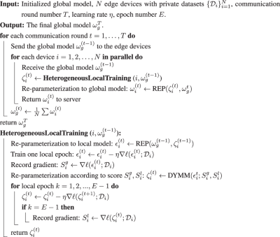
In this subsection, we elaborate the methodology of DynamicFL. We consider FL across N heterogeneous edge clients with diverse computational capabilities. Each client i can only access its own private dataset \({{{{\mathcal{D}}}}}_{i}=\{({{{{\bf{x}}}}}_{j}^{i},{y}_{j}^{i})\}\) where x and y denote the input features and corresponding class labels, respectively. The overall algorithmic workflow is summarized in 1 In the following, we elaborate the main steps of DynamicFL:
Initialization
Define the global model as the convolutional neural network, which is still widely used in real-world applications due to the advantage of parallel computing and lightweight memory footprint. The server initializes the model parameters and hyper-parameters and distributes the global model to all clients. In the first round, once the global model is received, the client i expands the K × K convolution layers to diverse branches adopted in DBB32 from bottom to top according to their computational resources:
We record the gradient of the last epoch as \({S}_{i}^{l}\), which reflects the sensitivity of each branch of the local model to local knowledge. The local model is then transformed back to the original plain structure and uploaded to the server. Since all uploaded local models have the same structure as the global model, we can perform the aggregation operation to derive the updated global model \({\omega }_{g}^{(0)}\).
Heterogeneous Local Training
The new global model is distributed to local clients, upon which the next round of local training is conducted. Considering local clients have diverse and limited computational resources, we dynamically adjust computational workloads by selecting operations that significantly contribute to performance, instead of re-parameterizing all candidate operations as done in DBB. The resource-adaptive models modulation is tailored according the local and global gradient information of FL. Specifically, in the t-th round, relying on the new global model \({\omega }_{g}^{(t-1)}\) and the stale local model \({\zeta }_{i}^{(t-1)}\) in the last round, we conduct structural re-parameterization to derive a temporary local model \({\epsilon }_{i}^{
(3)
where REP(⋅) represents the re-parameterization operation. We perform local training on \({\epsilon }_{i}^{
(4)
where \({S}_{i}^{g}\) reflects the sensitivity of each branch of the local model to the global knowledge, i.e., the aggregation result of all participants.
\({S}_{i}^{g}\) and \({S}_{i}^{l}\) offer useful cues to reflect the contribution of branches to the global aggregation. According to them, we dynamically evolve the network structures of the local model to remove redundant operations with little contribution while further expanding important operations with significant contribution, and obtain the new local model \({\zeta }_{i}^{
(5)
The details of DYMM(⋅) for how to use \({S}_{i}^{g},{S}_{i}^{l}\) to perform dynamic model modulation can be found in Section Dynamic Model Modulation.
Client i then performs local training along with its private data on the new local model \({\zeta }_{i}^{
(6)
where the number of epochs executed is E − 1, since one epoch has already been done in Eq. (4). The gradient information of the last epoch is recorded as the updated \({S}_{i}^{l}\):
It is worth mentioning a possible scenario: in this round, client i may have a smaller computational budget than in the last round due to other active routines, which makes it unable to afford the local model from the previous round. In this case, the steps correspond to Eq. (3), (4) and (5) cannot be performed. Instead, we conduct re-parameterization based on \({S}_{i}^{l}\) only to derive the new model:
$${\zeta }_{i}^{
(8)
Then, local training on \({\zeta }_{i}^{
(9)
\({\omega }_{i}^{
(10)
The equivalent transformations of operations during re-parameterization ensure lossless knowledge transfer across heterogeneous local models. The central server then distributes the new global model \({\omega }_{g}^{
Algorithm 1
Dynamic Federated Learning
Dynamic Model Modulation
In this subsection, we present the details of the DYMM( ⋅ ) operator to perform dynamic model modulation based on the local knowledge from the local private dataset and the global knowledge from the global aggregation.
We dynamically identify the important operations and redundant operations of local models according to the gradient information. Some works in the literature52,53 have shown that the gradient of each weight of the model in the training process can effectively reflect the sensitivity of the weight to data. Inspired by works54,55, we use the following metric to measure the salience of each weight:
Local knowledge in FL is easy to obtain during local training. In the (t − 1)-th round, we record the last local epoch gradient information by Eq. (7) and (11):
where θk is the k-th branch in the local model \({\zeta }_{i}^{(t-1)}\), and \({\theta }_{j}^{k}\) is the j-th parameter of the branch k. \({S}_{i}^{l}({{{{\boldsymbol{\theta }}}}}^{k})\) is leveraged for dynamic model modulation in the next round.
The global knowledge in FL is implicitly encoded into the global model, which is the aggregation result of all participating clients. To extract global information, according to the received global model \({\omega }_{g}^{(t-1)}\) in the t-th round and the last round local model \({\zeta }_{i}^{(t-1)}\), re-parameterization is conducted to get the temporary model \({\epsilon }_{i}^{t}\) through Eq. (3). Here \({\epsilon }_{i}^{t}\) is a re-parameterized model of \({\omega }_{g}^{(t-1)}\), which has the same structure as \({\zeta }_{i}^{(t-1)}\). We use \({\epsilon }_{i}^{t}\) to perform one-epoch local training with the private dataset, from which the derived gradient information reflects the sensitivity of the branches in the local model \({\zeta }_{i}^{(t-1)}\) to the global information:
where ψk is the k-th branch in the local model \({\epsilon }_{i}^{
(14)
where \({{{\psi }}}^{\left({{\rm{common}}}{\prime} \right)}\) is the new common branch after merging; ψ(common) and ψ(redundant) represent common and redundant branches, respectively. Then we expand the important branches to adapt the client’s computing capabilities:
where \({{{\psi }}}^{\left({{\rm{important}}}{\prime} \right)}\) are the expanded parameters of the important branch. In order to ensure the same output, we need to subtract the parameters of the new branch \({\{{{{\psi }}}^{(i)}\}}_{i=1}^{n}\) from the parameters of the original important branch ψ(important). The parameters of the new branch are generated randomly.
To ensure the stability and effectiveness of training, we adopt a fixed local reparameterization strategy for transformer-based models throughout the training process, unless computational resources change. Transformer architectures are particularly sensitive to parameter variations, and frequent changes to the reparameterization strategy may adversely affect their convergence and performance.
Lossless Knowledge Transfer
This section introduces the re-parameterization techniques for CNNs and transformers, demonstrating how these methods enable flexible structural transformations while preserving model outputs.
Re-parameterization for CNN
As indicated by works55,56, the 2D convolutions hold the property of additivity:
where I, F(1) and F(2) are the input and kernels, respectively. The above equation is satisfied even with different kernel sizes. Some widely used operations in CNN —- average pooling and batch normalization —- can be converted into a convolution operation. The above additivity property ensures that a single convolution can be equivalently transformed to multi-branch operations, and vice versa. The equivalent transformations of operations guarantee lossless knowledge transfer, since the model outputs are not changed along with the network structure adjustment.
Re-parameterization for Transformer
The re-parameterization technique can also be adapted to transformer architectures. In the case of transformers, the linear layers hold the property of additivity, similar to the convolution operation in CNNs:
where X is the input feature matrix, and W(1) and W(2) are the weight matrices of two linear layers. This equation implies that multiple parallel linear layers can be equivalently merged into a single linear layer, or vice versa.
Moreover, operations commonly used in transformer architectures, such as layer normalization and residual connections, can also be transformed into equivalent forms compatible with the re-parameterization technique. Specifically, layer normalization can be expressed as an affine transformation, which can be absorbed into the parameters of linear layers. Residual connections, being additive in nature, align naturally with the additivity property of linear operations.
The re-parameterization process for transformers involves expanding a single linear layer into multiple parallel linear layers, optionally combined with normalization layers (e.g., batch normalization or layer normalization). These parallel branches can then be merged back into a single equivalent linear layer without loss of information. This guarantees lossless knowledge transfer, as the outputs of the model remain unchanged before and after the structural reconfiguration:
where Wmerged is the weight matrix of the merged linear layer.
It is worth noting that, according to Eq. (16) and (17), the re-parameterization process in DynamicFL ensures mathematical equivalence between the original and transformed model structures, guaranteeing that the input-output mapping remains unchanged. As a result, when evaluating the model on the same test set, its accuracy remains identical, thereby ensuring fairness in the models obtained by institutions with different computational resources.
Convergence Analysis
In this subsection, we present the convergence analysis of DynamicFL. We consider the following standard assumptions commonly made in FL analysis57,58,59:
Assumption 1
(L-smoothness and σ-uniformly bounded gradient variance).
(a) F is L-smooth, i.e., \(F(u)\le F(x)+\left\langle \nabla F(x),u-x\right\rangle+\frac{1}{2}L{\left\Vert u-x\right\Vert }^{2}\) for any \(u,x\in {{\mathbb{R}}}^{d}\).
(b) There exists a constant Gmax > 0 such that: \({\mathbb{E}}(| | \nabla {F}^{(i)}(x)| {| }^{2})\le {G}_{max}^{2},\quad \forall i\in (N),\forall {{{\bf{x}}}}\in {{\mathbb{R}}}^{d}\), where ∇ F(i)(x) is an unbiased stochastic gradient of f(i) at x.
For any reparameterization of a convolutional layer l that can be represented as a summation of N convolutional branches with weights \({W}_{l,n}^{
(19)
where \({{{{\mathcal{G}}}}}_{l}={\sum }_{n=1}^{N}{M}_{l,n}\). Therefore, it can be seen as spatial gradient scaling applied to the original convolution. Here we assume \({{{{\mathcal{G}}}}}_{l}\le {{{\mathcal{G}}}}\). In FL, it can be expressed that for the local model \({\zeta }_{i,k}^{
(20)
Here, we note that the variable k denotes the current local epoch, and each client’s structure of \({\zeta }_{i,k}^{
(21)
This reparameterization ensures that the structure of ϕ
(22)
Theorem 3
The sequence generated by our method with stepsize η ≤ 1L satisfies
When the function f is lower bounded with \(f({w}_{1}^{(g)})-{f}^{*}\le \Delta\) and the number rounds T is large enough, then set the stepsize \(\eta=\frac{\sqrt{N}}{L\sqrt{T}}\) yields
The dominance of the first term in our algorithm ensures that it shares the same convergence speed, \(O(1/\sqrt{NT})\), as the vanilla FedAvg.
Statistics & Reproducibility
This study is based on a publicly available dataset. No statistical method was used to predetermine sample size. No data were excluded from the analyses. Since the dataset is pre-collected and publicly available, no randomization or blinding was applicable. The machine learning models were trained using standard procedures, and all experiments were conducted with fixed hyperparameters unless otherwise specified.
Reporting summary
Further information on research design is available in the Nature Portfolio Reporting Summary linked to this article.